Numerical integration - five techniques

In mathematics, integration is the opposite process to differentiation. Where differentiation can be used to find the rate of change of a curve, integration is commonly used to find the area under a curve, or the volume under a surface, or the equivalent in higher dimensions. Integration is also used to solve differential equations, amongst many other applications.
We know how to differentiate many different types of mathematical functions because we can often find derivatives from first principles. We can't generally integrate a function from first principles, so we can usually only find the integral of a function by applying what we know about derivatives. For example, if we know that differentiating f(x) results in g(x), we can determine (subject to certain conditions) that the integral of g(x) is f(x).
A consequence of this is that there are many functions that we cannot integrate analytically.
But sometimes we only need to know the approximate value of a definite integral (that is, the area under a curve between two points a and b). Numerical methods provide ways to calculate approximate integrals, often accurate to many significant figures, that are fine for most practical purposes.
This article will look at some of those methods:
Rectangular approximations
Trapezium rule
Simpson's rule
Monte Carlo methods
Integration by series expansion
Example
Here is a function f(x), and we wish to find an approximate value for the definite integral between x-values a and b:
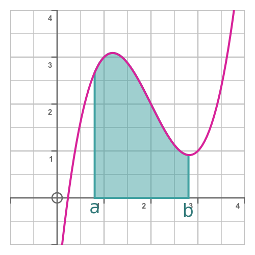
If we cannot integrate f(x) directly, we must look for an alternative solution. If we think of the problem in terms of calculating the approximate area under the curve, them we might consider a geoemetric approach. We will look at several approaches that can be used to calculate the area under almost any curve, perhaps to 6 signficant figures or better.
The function shown is:
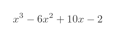
Of course, since this is a polynomial we can find its integral fairly easily, although for this article we will pretend we can't. The integral (ignoring the constant of integration) is:
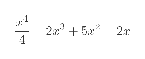
Before we go back to pretending we don't know this result, we will note that the integral between the range shown (0.8 to 2.8) is exactly 4.384. We can compare our approximate results to this exact value to see how well the approximations work.
Rectangular approximation
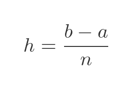
One possible approximation is to divide the area into n rectangles. We start by dividing the range a to b into n slices, each of width h:
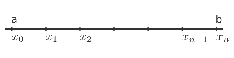
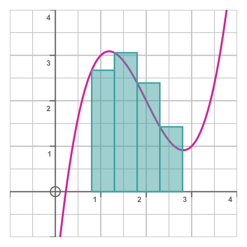
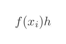
We have labelled the x-axis with n + 1 equally spaced values, where x0 is the start value, a, and xn is the end value, b. Now we can draw rectangles to approximate the area under the curve. Rectangle i starts at position xi, with height f(xi) and width h:
The width h is simply the distance from a to b, divided by n:
The area of rectangle i is given by:
We can see from the image that, provided the function behaves reasonably smoothly over the range, the total area of all the rectangles will be approximately equal to the area under the curve. To illustrate the technique, we have only used four slices, so it is easy to see how the area of the slices differs from the area under the curve. But a computer would easily be able to calculate thousands or even millions of slices in a very short time, giving quite an accurate estimate of the true area (see below).
The total area of all the rectangles is:
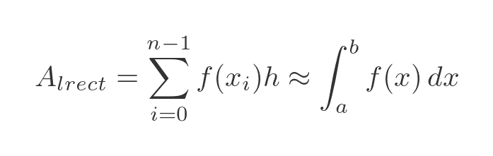
We have labelled this the lrect area because it is formed from rectangles whose height is given by the value of the function at the left-hand bound of the rectangle.
How accurate is this approximation? Recall that the exact area is 4.384. The approximate results (to four decimal places) are:
4 slices: 4.7740
1000 slices: 4.3857
Not surprisingly, 4 slices give a fairly inaccurate result. 1000 slices is correct to almost three dp.
Alternative rectangle form
We could draw the rectangles in a slightly different way, like this:
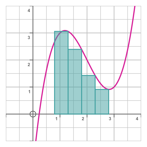
This time the height of each rectangle is given by the value of the function at the right-hand bound of the rectangle, so we will call this the rrect area. It is calculated using this slightly different formula:
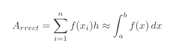
All we have done here is let the summation count from 1 to n, rather than 0 to n - 1 as before. This means that the first rectangle has a height of f(x1) rather than f(x0), and similar for all the other terms.
The new results are:
4 slices: 3.8940
1000 slices: 4.3822
The lrect area and the rrect area are always likely to be slightly different. Depending on the curve and the position of the endpoints, one or the other might be more accurate. However, there is a simple technique for getting the best of both worlds, as we will see next.
Trapezium rule
Rather than trying to model the area using rectangles, we could try using trapezium shapes, like this:
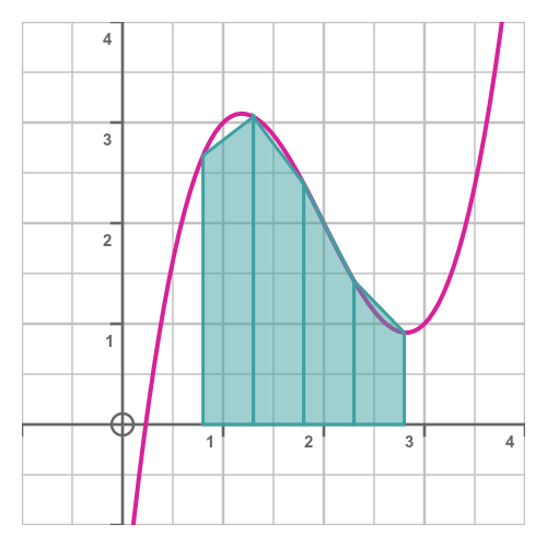
This looks like it fits the curve much more accurately, so we would expect a more accurate result.
